The Trade-Off Between Accuracy and Agreement in AI Models
Table of Links
Abstract and 1. Introduction
1.1 Post Hoc Explanation
1.2 The Disagreement Problem
1.3 Encouraging Explanation Consensus
-
Related Work
-
Pear: Post HOC Explainer Agreement Regularizer
-
The Efficacy of Consensus Training
4.1 Agreement Metrics
4.2 Improving Consensus Metrics
[4.3 Consistency At What Cost?]()
4.4 Are the Explanations Still Valuable?
4.5 Consensus and Linearity
4.6 Two Loss Terms
-
Discussion
5.1 Future Work
5.2 Conclusion, Acknowledgements, and References
Appendix
4.1 Agreement Metrics
In their work on the disagreement problem, Krishna et al. [15] introduce six metrics to measure the amount of agreement between post hoc feature attributions. Let [𝐸1(𝑥)]𝑖 , [𝐸2(𝑥)]𝑖 be the attribution scores from explainers for the 𝑖-th feature of an input 𝑥. A feature’s rank is its index when features are ordered by the absolute value of their attribution scores. A feature is considered in the top-𝑘 most important features if its rank is in the top-𝑘. For example, if the importance scores for a point 𝑥 = [𝑥1, 𝑥2, 𝑥3, 𝑥4], output by one explainer are 𝐸1(𝑥) = [0.1, −0.9, 0.3, −0.2], then the most important feature is 𝑥2 and its rank is 1 (for this explainer).
\ Feature Agreement counts the number of features 𝑥𝑖 such that [𝐸1(𝑥)]𝑖 and [𝐸2(𝑥)]𝑖 are both in the top-𝑘. Rank Agreement counts the number of features in the top-𝑘 with the same rank in 𝐸1(𝑥) and 𝐸2(𝑥). Sign Agreement counts the number of features in the top-𝑘 such that [𝐸1(𝑥)]𝑖 and [𝐸2(𝑥)]𝑖 have the same sign. Signed Rank Agreement counts the number of features in the top-𝑘 such that [𝐸1(𝑥)]𝑖 and [𝐸2(𝑥)]𝑖 agree on both sign and rank. Rank Correlation is the correlation between 𝐸1(𝑥) and 𝐸2(𝑥) (on all features, not just in the top-𝑘), and is often referred to as the Spearman correlation coefficient. Lastly, Pairwise Rank Agreement counts the number of pairs of features (𝑥𝑖 , 𝑥𝑗) such that 𝐸1 and 𝐸2 agree on whether 𝑥𝑖 or 𝑥𝑗 is more important. All of these metrics are formalized as fractions and thus range from 0 to 1, except Rank Correlation, which is a correlation measurement and ranges from −1 to +1. Their formal definitions are provided in Appendix A.3.
\ In the results that follow, we use all of the metrics defined above and reference which one is used where appropriate. When we evaluate a metric to measure the agreement between each pair of explainers, we average the metric over the test data to measure agreement. Both agreement and accuracy measurements are averaged over several trials (see Appendices A.6 and A.5 for error bars).
4.2 Improving Consensus Metrics
The intention of our consensus loss term is to improve agreement metrics. While the objective function explicitly includes only two explainers, we show generalization to unseen explainers as well as to the unseen test data. For example, we train for agreement between Grad and IntGrad and observe an increase in consensus between LIME and SHAP.
\ To evaluate the improvement in agreement metrics when using our consensus loss term, we compute explanations from each explainer on models trained naturally and on models trained with our consensus loss parameter using 𝜆 = 0.5.
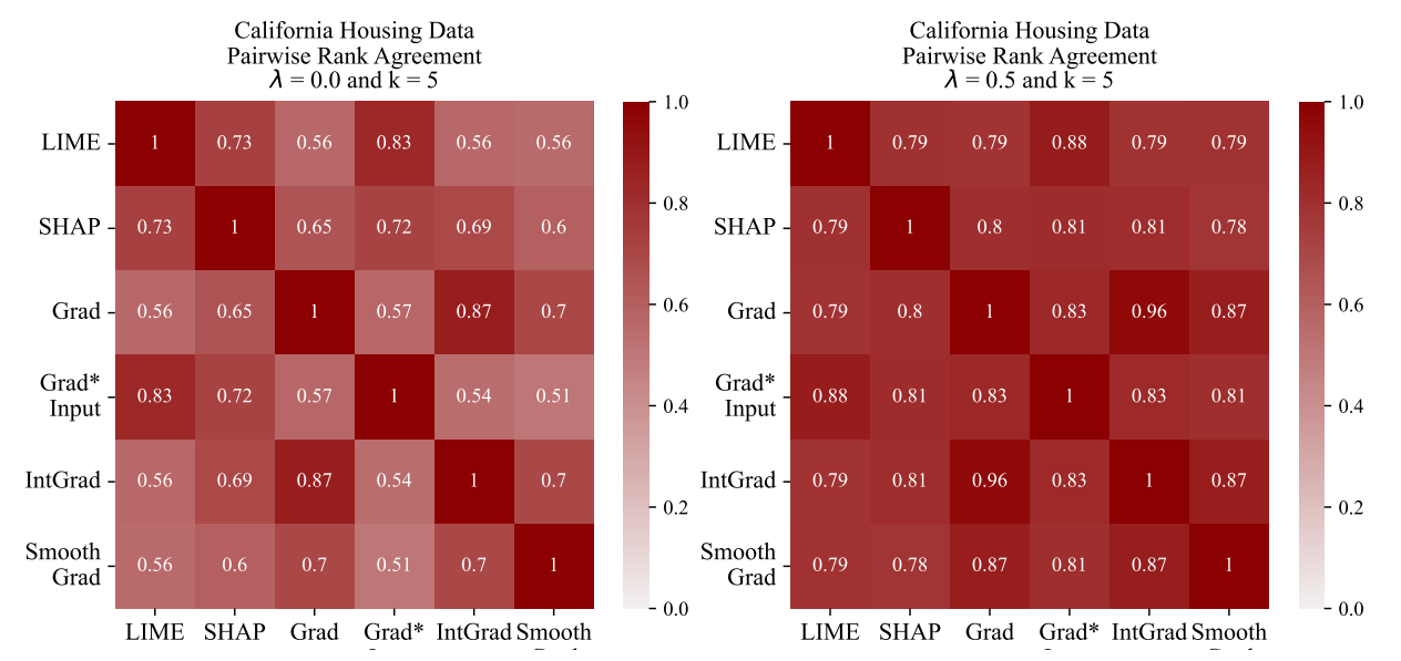
\ In Figure 4, using a visualization tool developed by Krishna et al. [15], we show how we evaluate the change in an agreement metric (pairwise rank agreement) between all pairs of explainers on the California Housing data.
\ Hypothesis: We can increase consensus by deliberately training for post hoc explainer agreement.
\ Through our experiments, we observe improved agreement metrics on unseen data and on unseen pairs of explainers. In Figure 4 we show a representative example where Pairwise Rank Agreement between Grad and IntGrad improve from 87% to 96% on unseen data. Moreover, we can look at two other explainers and see that agreement between SmoothGrad and LIME improves from 56% to 79%. This shows both generalization to unseen data and to explainers other than those explicitly used in the loss term. In Appendix A.5, we see more saturated disagreement matrices across all of our datasets and all six agreement metrics.
4.3 Consistency At What Cost?
While training for consensus works to boost agreement, a question remains: How accurate are these models?
\ To address this question, we first point out that there is a tradeoff here, i.e., more consensus comes at the cost of accuracy. With this in mind we posit that there is a Pareto frontier on the accuracy-agreement axes. While we cannot assert that our models are on the Pareto frontier, we plot trade-off curves which represent the trajectory through accuracy-agreement space that is carved out by changing 𝜆.
\ Hypothesis: We can increase consensus with an acceptable drop in accuracy
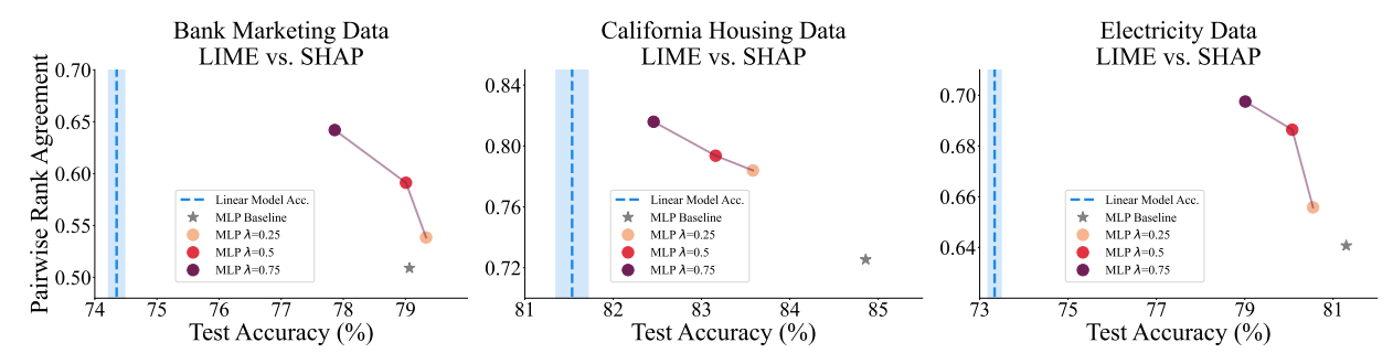
\ While this hypothesis is phrased as a subjective claim, in reality we define acceptable performance as better than a linear model as explained at the beginning of Section 4. We see across all three datasets that increasing the consensus loss weight 𝜆 leads to higher pairwise rank agreement between LIME and SHAP. Moreover, even with high values of 𝜆, the accuracy stays well above linear models indicating that the loss in performance is acceptable. Therefore this experiment supports the hypothesis.
\ The results plotted in Figure 5 demonstrate that a practitioner concerned with agreement can tune 𝜆 to meet their needs of accuracy and agreement. This figure serves in part to illuminate why our
\ 
\ 
\ hyperparameter choice is sensible—𝜆 gives us control to slide along the trade-off curve, making post hoc explanation disagreement more of a controllable model parameter so that practitioners have more flexibility to make context-specific model design decisions.
\
:::info Authors:
(1) Avi Schwarzschild, University of Maryland, College Park, Maryland, USA and Work completed while working at Arthur (avi1umd.edu);
(2) Max Cembalest, Arthur, New York City, New York, USA;
(3) Karthik Rao, Arthur, New York City, New York, USA;
(4) Keegan Hines, Arthur, New York City, New York, USA;
(5) John Dickerson†, Arthur, New York City, New York, USA ([email protected]).
:::
:::info This paper is available on arxiv under CC BY 4.0 DEED license.
:::
\
You May Also Like

Solana ETFs Market Grows with Fidelity and Canary Marinade’s New Funds

XRP analysts shift 2025 outlook as liquidity models evolve